MEAP Tutorial

Part I: Preprocessing Your Data

Step 1: Creating your Input File

Note

MEAP also allows the user to input individual files one-by-one. However, when batch processing data we recommend creating an input file as specified below. For more on importing files individually, see Step 2: Importing & Mapping the Channels below.

The first step is to create an input file that tells MEAP where the data you want to analyze is stored. MEAP can accomodate both AcqKnowledge (.acq) and matlab (.mat) files. Each file should contain the cardiovascular reactivity data collected from one participant including electrocardiogram (ECG), impedance (IKG), blood pressure (BP) waveforms , and respiration (optional). Data must be collected continuously and sampled at at least 1,000 HZ.

Warning

DON’T USE COMMAS IN YOUR FILE NAMES

In addition to the data file(s) you are scoring, you will need to create a comma separated text file (.csv) or excel file (.xlsx) that contains the path to each data file to be scored. This file will be used to import the data for initial preprocessing. Later you will create a design file that contains information specific to your experimental design and analysis method. This initial input file MUST contain the columns containing the following information labeled as such:

1. File - specify the full path to each file to be scored

2. Inter-electrode distances-

   1. When using a mylar band configuration label columns:

   electrode_distance_front - the distance between impedance electrodes on the front of the torso.

   electrode_distance_back - the distance between impedance electrodes on the back of the torso.

   2. When using a spot electrode configuration label columns:

   electrode_distance_left

   electrode_distance_right and enter the corresponding measurements.

Note

All measurements must be in centimeters.

For a complete list of input file options see Participant Parameters.

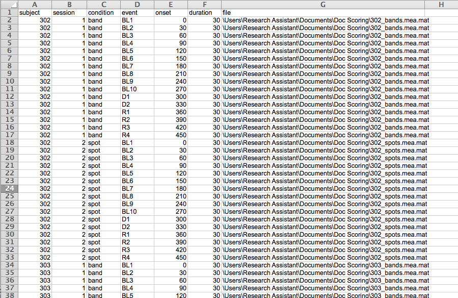
Here is an example input file:

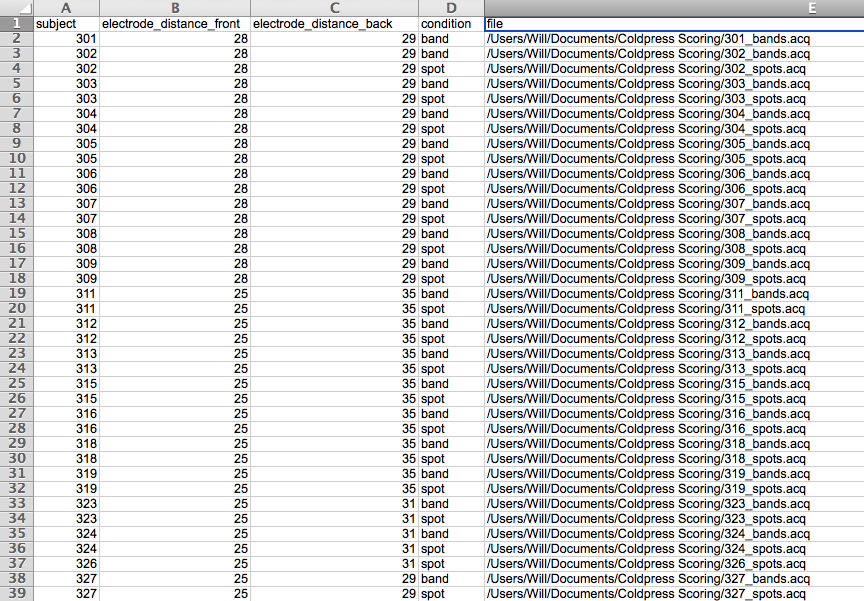
To add the file paths more quickly create columns for study condition, task, and any other variables relavant to your design. Name your Acknowlege files based on these values and use excel’s CONCATENATE function to populate the file path. For example, here the path for the first row of data is CONCATENATE = (“/Users/Will/Documents/Coldpress Scoring/”, A2, “_”, D2, “s.acq”). Simply drag this equation down the column to populate the rest of the file paths.

Warning

If you have a lot of data, it may be best to create several smaller input files with only a subset of your participants or cases. This will reduce the amount of data that MEAP has to load at one time and can prevent the program or your computer from crashing or running slowly.

Step 2: Importing Data & Mapping the Channels

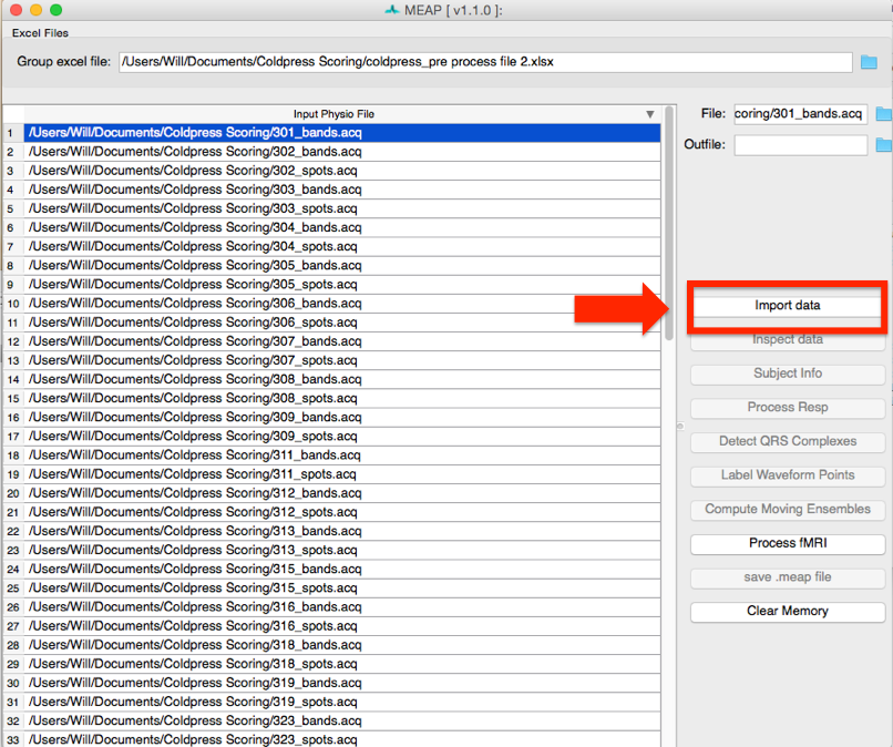
When you launch MEAP, you will see a window that looks like this:

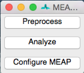
Select Preprocess. This will open a window that looks like this:

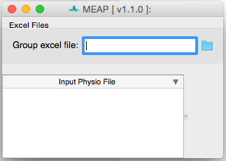
Click on the folder in the upper right corner to navigate to your input file. Information from this spreadsheet will be called and a window will appear that contains all of your files to be scored and also serves as the primary user interface.

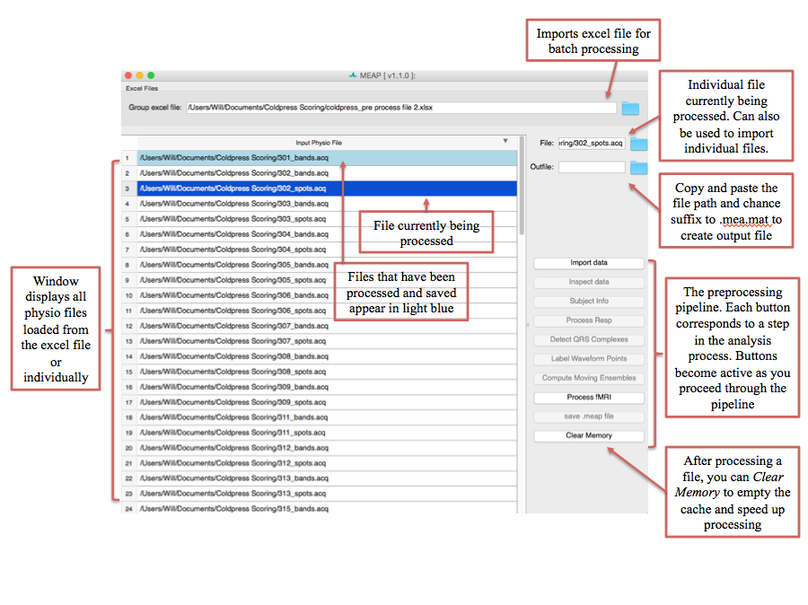
Files to be processed appear in white. Once you finish the preprocessing pipeline and save as .mea.mat file, the row will turn light blue. The file currently being processed appears in dark blue. To import files individually, right click within the “Input Physio file” portion of the window and select Add New Item. Then click within the blank line that appears and then navigate to the file you wish to score using the blue folder icon to the right of the File field.

Now select the first file you would like to process. Then click on the Import data button at the right of the screen to begin preprocessing.

Once your Aqcknowledge file is imported you’ll need to let MEAP know which channel contains each data source. If loading from a mea.mat file, the channels have already been stored. For Acqknowledge files, specify the data contained within each channel using this GUI:

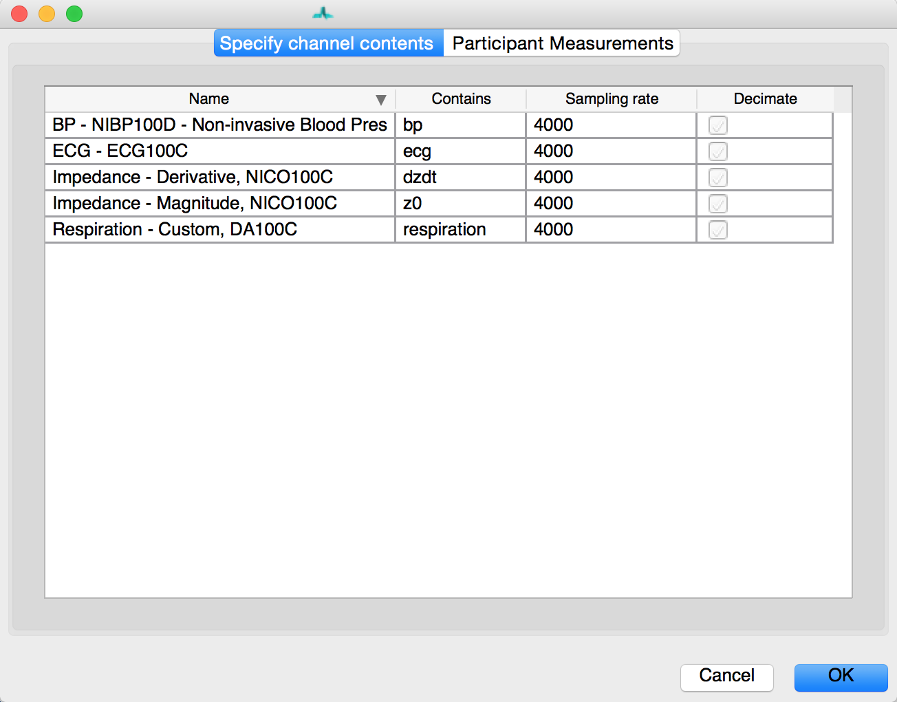
The channel names from your data file appear on the left. Match these with the data types specified in the dropdown menus on the right. If blood pressure data was collected using a wireless blood pressure system or other system that generates separate channels for diastolic and systolic blood pressure, map each of these accordingly; systolic and diastolic are both options in the drop down menu. Any remaining channels that you do not wish to import data from should be set to None.

Regardless, of the number of channels that appear in the .acq file and their names, you should have the following channels mapped:

1. ECG - Electrocardiogram data
2. z0 - Magnitude of impedance
3. bp - Blood pressure (or systolic and diastolic; optional)
4. dzdt - First derivative of impedance magnitude.
5. respiration- breath data (optional)
6. doppler - Cardiac doppler radar signal (optional)

This window also contains a tab in which you can specify or correct the participant’s measurements. The inter-electrode distances are imported directly from your input file as is any other information you specified including height, weight, respiration circumference, and whether data was collected during Magnetic Resonance Imaging (MRI). This latter specification in critical as MEAP utilizes a customized point-marking algorithm for data collected within the scanner.

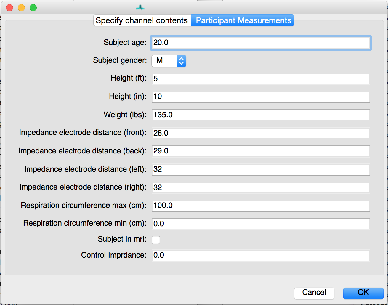
When importing files individually you MUST manually enter the participant measurements here. These values can also be edited after the fact by clicking on the Subject Info button.

For more information on these parameters and how to specify them in your input file see Participant Parameters.

Step 3: Check the Quality of Your Waveforms

Now that you have specified the type of data contained within each channel and updated participant measurements as desired, click on the Inspect data button at the bottom of the GUI.

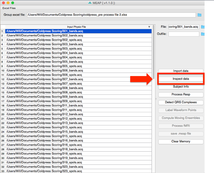
MEAP will load and display the data in a GUI like this:

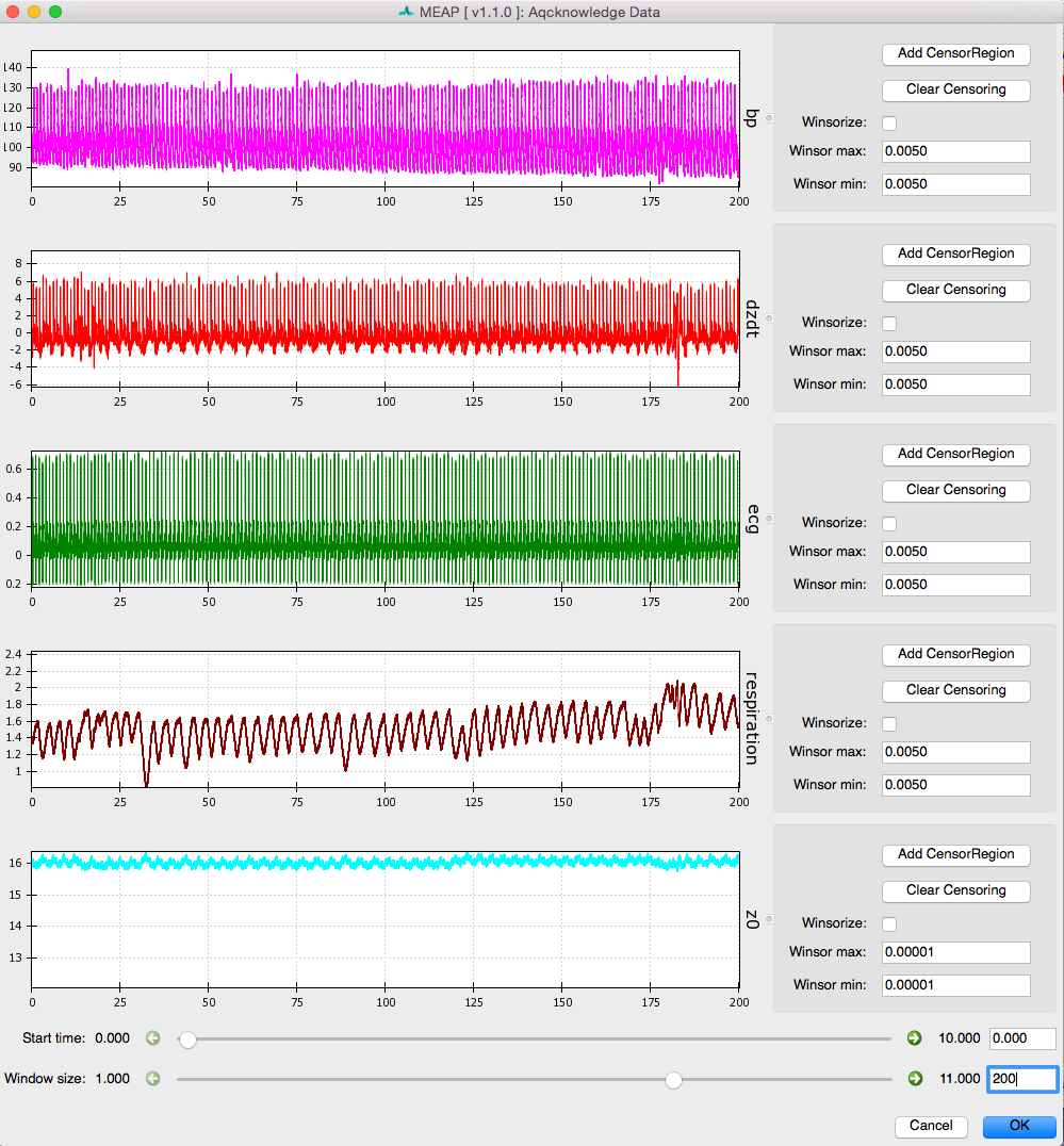
This feature is designed to allow the user to check the quality of the data, remove outliers, and flag any segments of data that contain noise or artifacts or that the researcher would like to exclude from analyses for whatever reason. Flagged sections will then be removed from all future analysis steps including point marking and ensemble or moving ensemble averaging.

Warning

It is critical that all data included in calculations be as clean as possible. Attempting to analyze data with significant artifacts will not yield interpretable values.

Windsorizing: Removing Extreme Outliers

The first thing to do when inspecting your data is to Windsorize outliers, if necessary. For example, the Z0 signal may drop to zero at the beginning or end of a file leading the wave form to appear small and uncentered in the window, as shown in image above. Such extreme outliers can be removed by selecting the Windsorize button next to the waveform that contains outliers and setting the maximum and minimum cutoffs for outliers. For example, setting both the max and min values to .005 means that you are pulling in the top and bottom 0.5% of the data to just inside that cutoff. You may need to adjust one or both of these parameters depending on the outliers contained within your data. Ideally, you want to set these cutoffs so that you are removing only extreme outliers and not any meaningful data. If Windsorizing leads to your waveforms appearing truncated, set lower cutoff values. If you don’t see your window update, check and uncheck the Windsorize button for that waveform.

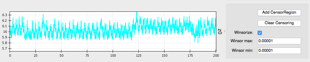
Post-windsorizing your Z0 data should look like this:

Censor Regions: Removing Noise & Aritfacts

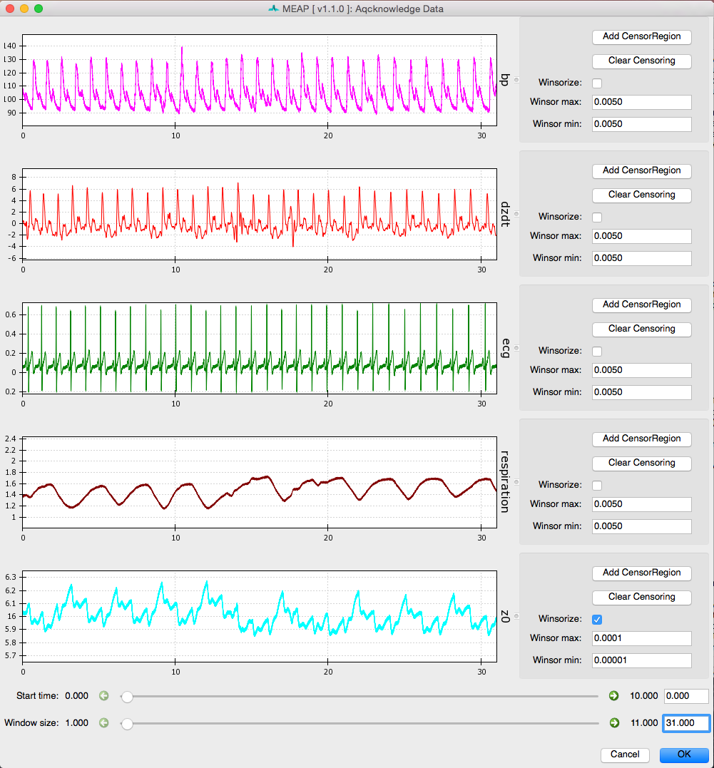
Next, use the Window size slider at the bottom of the screen to select a widow size that optimizes viewing your data. We recommend a window size of between 20 and 60 seconds to allow the user to clearly visualize each waveform and inspect it for anomalies.

Like so:

Using the Start time slider you can scroll through the length of your data file. You’ll notice that if you start at time 0 and move the slider to the far right, you do NOT reach the end of the file (unless it is very short). To do this you must use the green arrows to increase the sensitivity of the slider by a factor of 10 each time. Alternatively, you can jump to a specific time point by entering it into the box to the right.

As you scroll through, look for any sections where the waveform deviates significantly from it’s canonical shape.

Artifacts can look like this, where the signal drops off or shoots up beyond expected values:

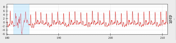
Artifacts can also look like this, where the signal deviates from its canonical shape, although values do not appear out of bounds:

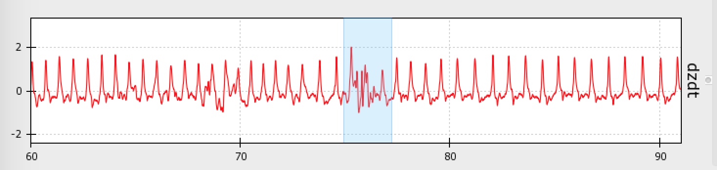
Artifacts are most likely to occur in the dz/dt signal, but may occur in any of the data streams.

Note

For more info on what wave forms should look like, see Physiological Data: Waveforms & Inflection Points

Whenever you come across an area of noise like this, you will want to remove it from analyses by censoring it out. This is accomplished using the Censor buttons to the right of each signal. Select the button that matches the waveform you wish to edit and use your curser to highlight the region you would like to exclude. If you would like to remove multiple regions, simply click on the Censor dz/dt again and select another region. To censor regions on additional waveforms, simply select the relevant Censor button and highlight the region.

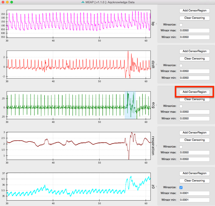
Do this as necessary for each waveform. If a region is censored out on one waveform (the dz/dt wave, for example) this same time interval is censored out of all other waves as well. Therefore, if artifacts occur in multiple waveforms simultaneously, it is not necessary to censor them separately on each waveform (as in the image above). This means that if one signal is bad throughout it is best not to edit this out, but to leave it and remove calculated values later in the analysis pipeline. For example, if BP data is bad throughout this approach will allow you to still analyze the impedance and ECG data. Without good ECG data, however, MEAP cannot calculate and align cardiac cycles and analysis will not be possible.

Note

This editing feature can also be employed to remove epochs of data that the researcher does not wish to include in analyses.

Once you are satisfied with the regions to be removed, select OK.

This is a good time to save your work. To do so, copy the File path and paste it into the Outfile field and change the file type from .acq to .mea.mat, then click Save .meap file. You could also provide any file name as long as it ends with .mea.mat.

Step 4: Processing Respiration Data

If you collected respiration data as part of your study MEAP can calculate the number of breaths. MEAP can also calculate breath rate from the ICG data. Additionally, by processing respiration in this way the user can remove the low frequency fluctuation in ICG signals due to respiration rather than changes in blood flow. Because the torso expands with each inhalation, the respiration cycle impacts impedance data in ways that may or may not be of interest to the researcher.

Select Process Resp:

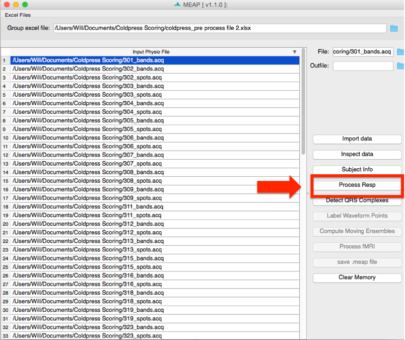
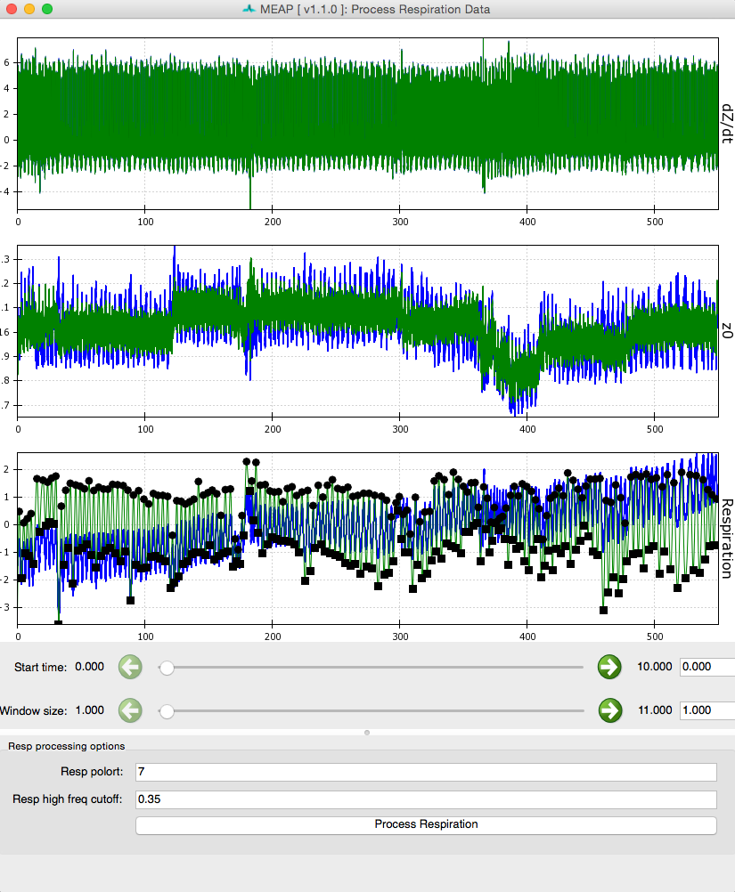
This will load a window like the one below which shows dz/dt, Z0, and respiration waveforms.

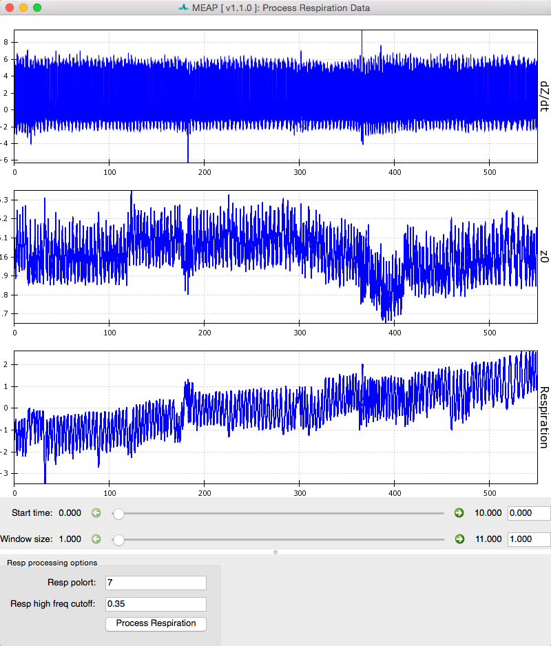
Click the Process Respiration button at the bottom of the screen and MEAP will use either the measured respiration signal or low frequency components of the ICG wave to determine respiration rate and remove its influence on the dz/dt and Z0 waveforms. The blue lines represent raw data and green represents data with variation due to respiration removed. Black dots mark inhalation and exhalation.

Sliders can be used to change the size and start point of the viewing window just like at the Inspect Data step.

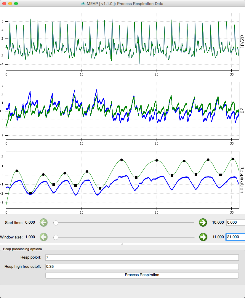
Processed respiration using measured respiration signal:

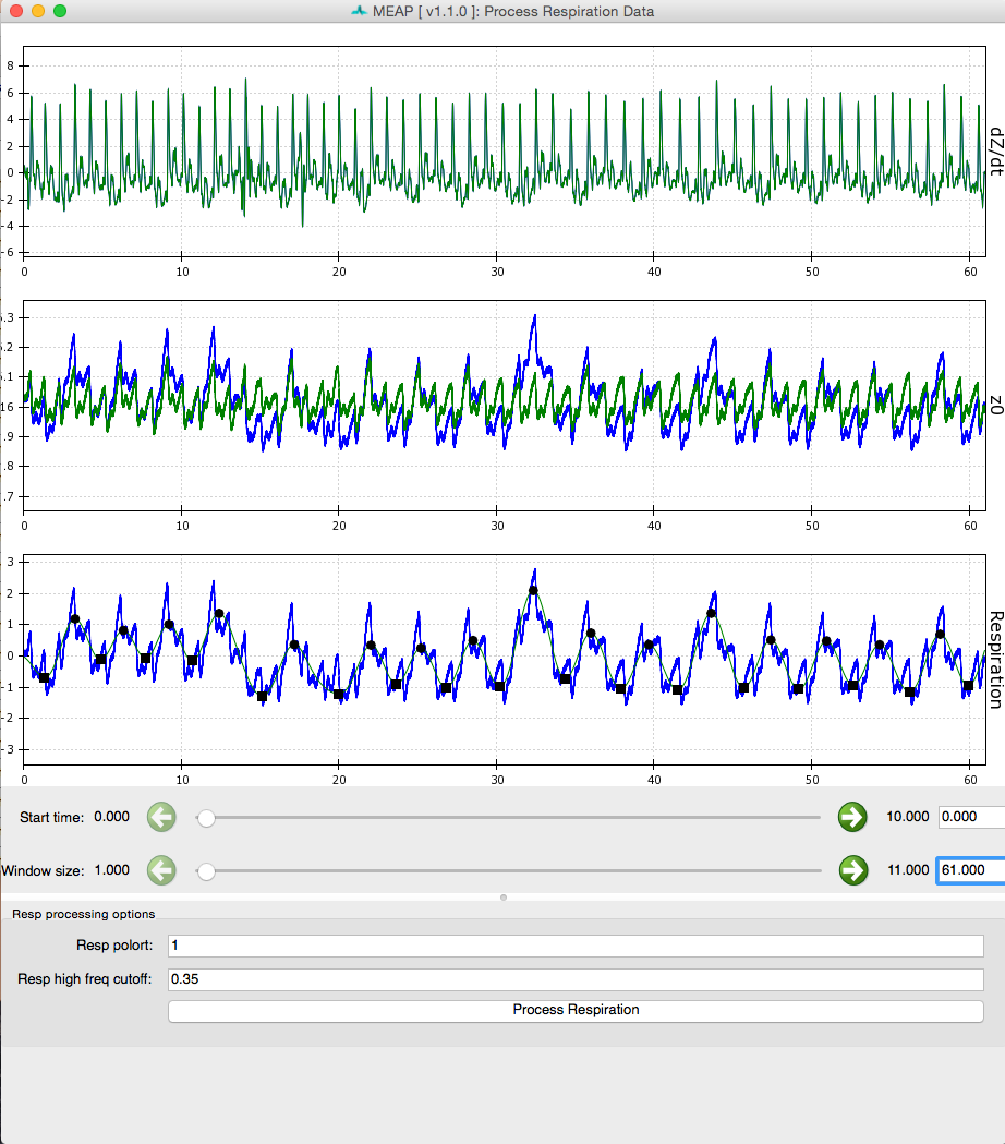
Processed respiration using dz/dt waveform:

After respiration has been processed, simply close the window and proceed to the next step.

Respiration correction is a very useful preprocessing step. Consider the Kubicek equation for calculating stroke volume. The Z0 term is directly included, which means that respiration-related signals will be incorporated in stroke volume and impact all measurements that use stroke volume. These include cardiac output and TPR. One remedy to respiration artifact is ensemble averaging. However, unless the same portions of the respiratory cycle are included in each time window, respiration-driven changes will only add to your model’s noise term.

Step 5: Detecting R-Peaks

Now that you have loaded your data, checked its quality, and removed areas of artifact, the next step is to detect each heartbeat. Click on the Detect QRS Complexes button.

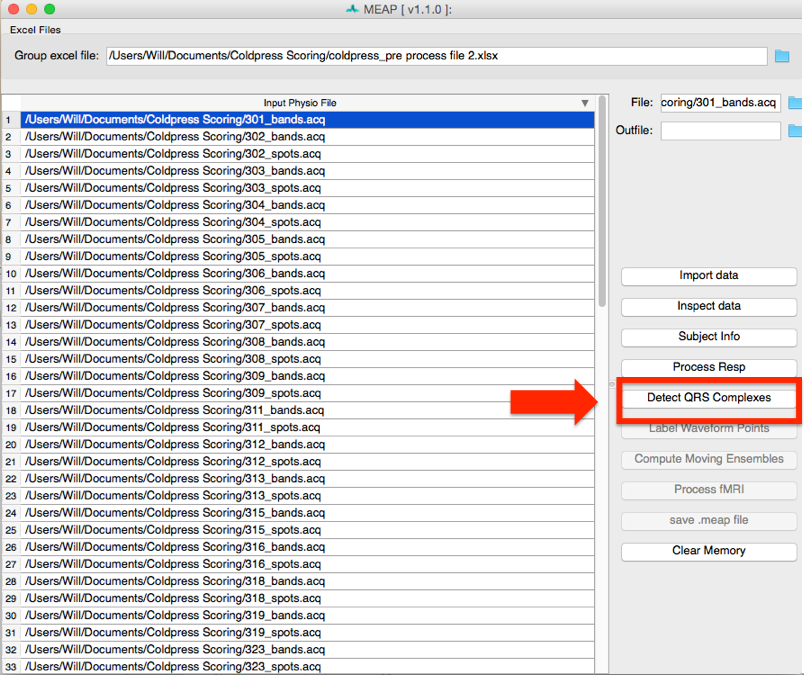
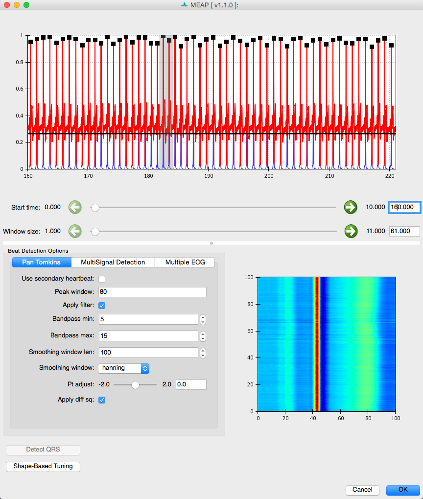
MEAP automatically detects each R-peak using a modified Pan-Tomkins algorithm (for more information on the Pan-Tompkins method see Beat Detector). There are other options for QRS detection that work better for data collected in an MRI scanner. However, all methods share the same basic editing tools.

Each R peak on the ECG wave is marked with a black square.

Again, the sliders below the displayed data allow the user to scroll through the file and change the window size.

If you censored any ECG data in the previous step, the R-peaks that fall within this region will be ignored. R-peaks in regions censored due to noise in other signals will still be detected.

The bottom right corner of this window displays a topographical image of all detected R-peaks. This image displays all R-peaks aligned with one another and viewed from above. The peak of each waveform appears in red while troughs appear in blue. This image allows the user to easily visualize the data and whether R-peaks have been correctly detected. When R-peaks are incorrectly marked, this image will apear jumbled rather than stripes of color corresponding to the topography of the canonical ECG waveform.

In most cases the default settings will allow for accurate detection of each R-peak. Depending on the noisiness of the data and/or idiosyncratic differences in waveform shape, however, the user may need to adjust the default settings. Adjustments are usually required only where a participant has a very high t-wave or where there is significant respiration or other artifact.

The beat detector GUI allows the user to edit the parameters of a modified Pan Tomkins QRS detector in order to more accurately mark the R-peaks in cases such as those just described. The most likely change you will need to make is to change the Pt adjust setting to be slightly higher or lower. If it is falsely detecting t-waves as peaks, adjust it up, if true R-peaks are being missed, adjust it down. Usually a change of .05 to .1 does the trick. Don’t forget if you sensored regions previously, R-peaks that fall within these regions will not be marked.

If there is an R-peak that is incorrectly marked due to noise that you missed in the previous step, you can remove this point now. Hold down the right-click button and mouse over the R-peaks you wish to delete, then right click again within that region to remove those point markings.

Simply click within the portion of the window displaying each R-peak. The squares marking these will change from black to yellow. Use the mouse to highlight the are surrounding any points you want to remove (just like in the edit data step above.

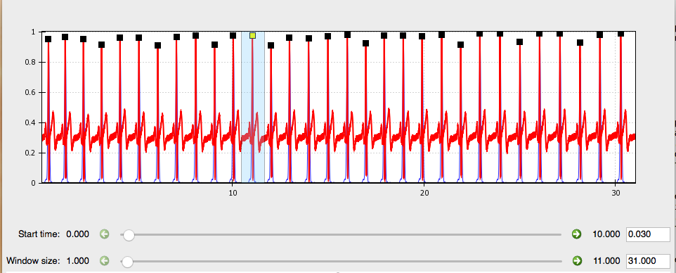
You can also mark individual R-peaks as needed by highlighting the peak you wish using the left-click button on your mouse.

Note

For more information on the Pan-Tompkins method and parameter options, see the Beat Detector section of this documentation.

Step 5a: Finding QRS complexes in the MRI

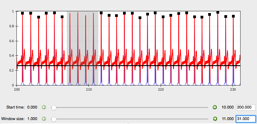
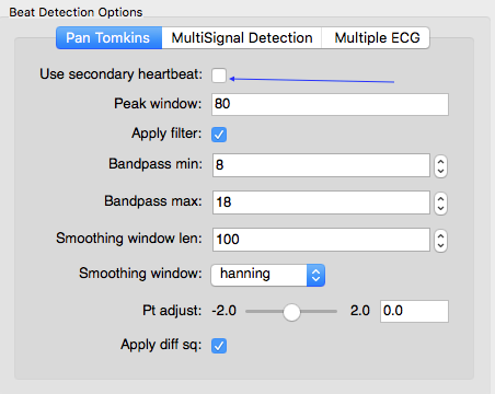
The ECG signal is much noisier in the MRI scanning environment. This is due to a number of factors, including magnetohydrodynamics (the effect of the magnetic field on blood) and RF noise from the scanner. One option is to use a second signal that captures some aspect of the cardiac cycle that is less impacted by scanner noise, such as dZ/dt or a pulse oximiter. We call this Multi Signal Detection. To enable Multi Signal Detection, check this box:

Select which signal you want to use as the secondary cardiac cycle indicator

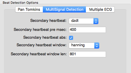
and indicate how to filter this signal. Ideally there should be a single local maximum corresponding to each heart beat. The secondary signal gets low-pass filtered according to these options and peaks are identified. Then a search window is built around each peak and an attempt is made to identify a QRS complex within each search window:

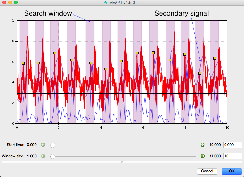
The search windows are light purple and highlight the area around peaks in the secondary signal. In this instance dZdt is the secondary signal, so the window is placed in front of its peaks (because the QRS precedes the peak of dZ/dt). QRS complexes identified in this way can still be edited using the same clicking tools described above.

Step 6: Marking Custom Points

The next step is to provide MEAP with information about where to look for inflection points of interest in this subject’s file.

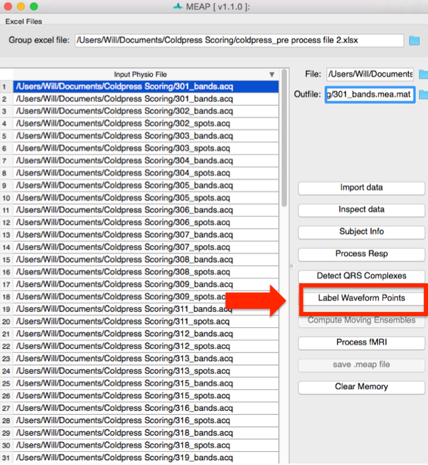
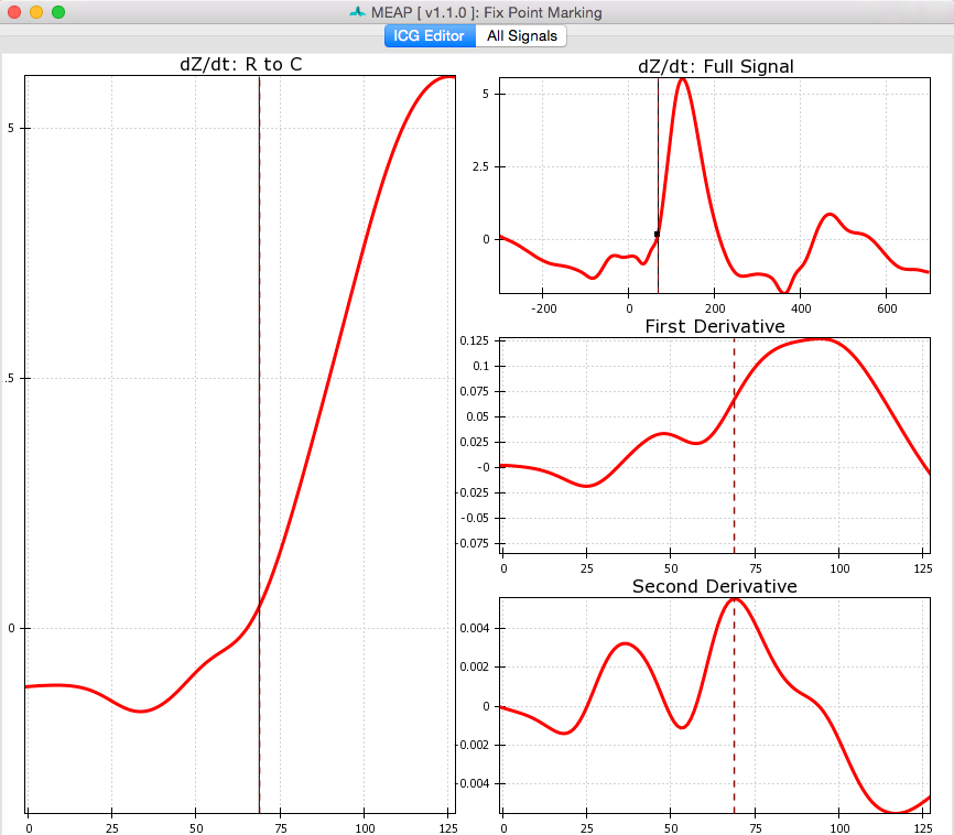
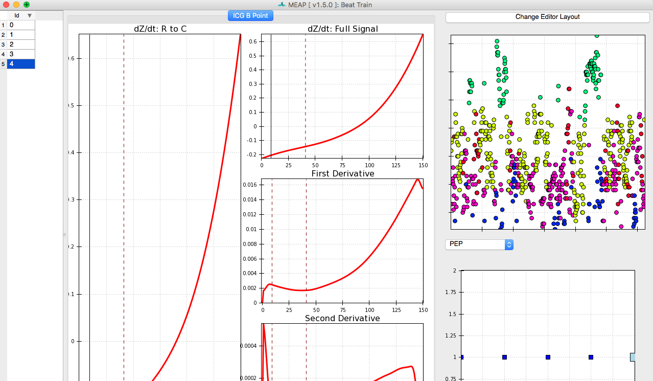
Clicking the Label Waveform Points button brings up a window displaying an ensemble averaged waveform for the entire data file. The ICG Editor tab shows the dz/dt wave produced by ensemble averaging the entire file (excluding any censored regions). The full dz/dt signal as well as it’s first and second derivatives are displayed along side a zoomed-in view of the R to C portion of the dz/dt wave. These features are designed to assist the user in selecting the B-point on the ensemble averaged waveform. By hovering over any of these images, the dashed line indicating the b-point crossing can be adjusted to the desired position.

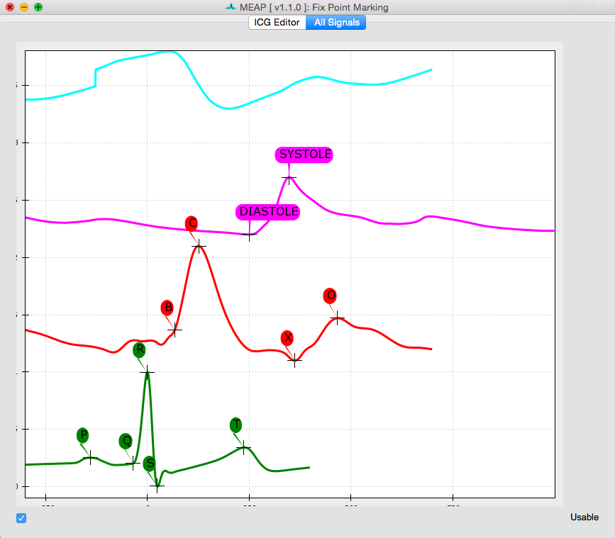
The All Signals tab displays the ensemble averaged waveforms for all physiological signals (except respiration) across the entire .acq file. Using a classifier derived from previous data, MEAP has attempted to mark each of the relevant inflection points on this waveform. It is the job of the user to examine these points, determine whether each is marked in the correct location, and to adjust their placement where necessary. Point markings can be adjusted by simply clicking on each and dragging it to the correct location. Moving the B-point in either of the two tabs adjusts its placement in the other. Correct point markings should look like this:

Warning

If you cannot find where one of the points is marked, it may be hidden beneath one of the other points. Occasionally with messy data one point will be placed on top of one another such that one is not visible.

Once each point is marked on the ensemble averages, MEAP will use these values to update it’s classifier and determine where to look for and mark the corresponding points at each individual ensemble average or beat (depending on type of analysis).

When you are satisfied with the placement of each point on the heuristic ensemble average, simply close the window and proceed to the next step.

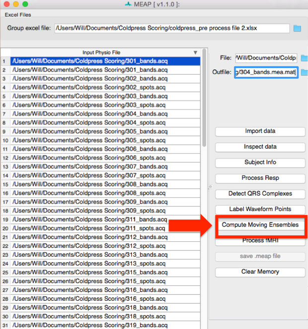
Step 7: Compute Moving Ensembles

The next step is to compute moving ensemble averages.

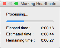
It takes some processing power for MEAP to use its classifier to compute the moving ensembles and mark relevant points on each ensembled beat. While it’s processing you will see a window like this:

When it’s done you will see a window like this:

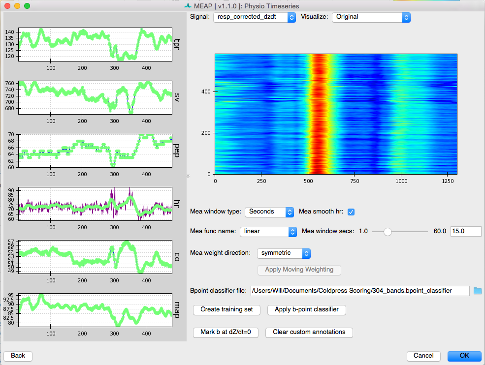
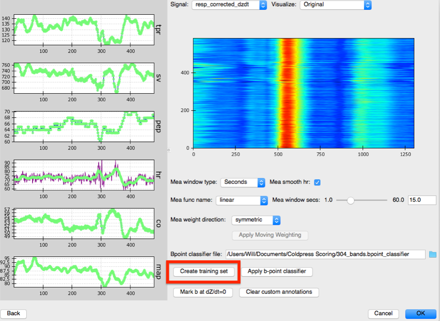
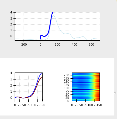
Along the left panel are displayed each of the main physiological indices MEAP computes plotted as a time series. In green are the values as calculated using the moving ensemble average. The purple trace indicates what these values would be using just the raw data.

The right panel displays a topographical map of the raw dz/dt data corrected for respiration. Changing the setting for Signal allows the user to view each of the different data streams in this manner. The Visualize option allows the user to select to view the raw or Original data, the data after the moving ensemble average is applied, or the residuals of this moving ensemble analysis.

Moving Ensembled:

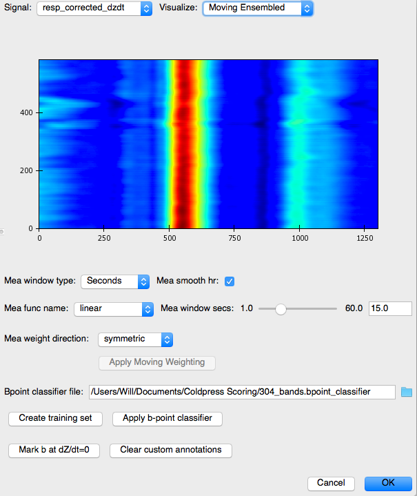
Note, how much cleaner the moving ensemble is than the raw data.

Residuals:

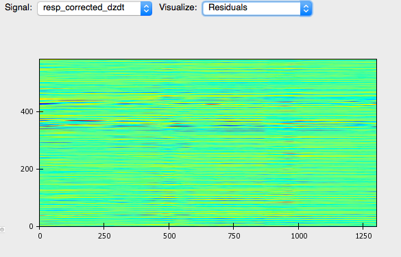
Ideally, residuals will be random, producing no clear pattern in the image.

Identifying B-Points

The most time-consuming and error-prone part of ICG analysis is identifying B-Points. This is a critical time for determining systolic intervals and therefore great care should be taken when marking this point.

MEAP provides two methods for automating this process. The first, an AdaBoost-based B-Point classifier was described in our 2018 Psychophysiology paper. This approach works very well, but requires manually labeling hundreds of points per recording to train the classifier. The second is unpublished, but relies on time series registration to “warp” B-points from a set of ICG shape templates. This method is much faster and has nice theoretical properties.

Training the B-Point Classifier

B-points are notoriously difficult to mark as they are neither a maximum or a minimum. Thus, although we have provided a prior to MEAP to tell it where to look for the b-point, we want to provide MEAP with more data with which to train its b-point classifier. To do this click on: Create Training Set. With this button press, MEAP will randomly select a number of beats from the file (the default is 100 beats) for the user to hand mark.

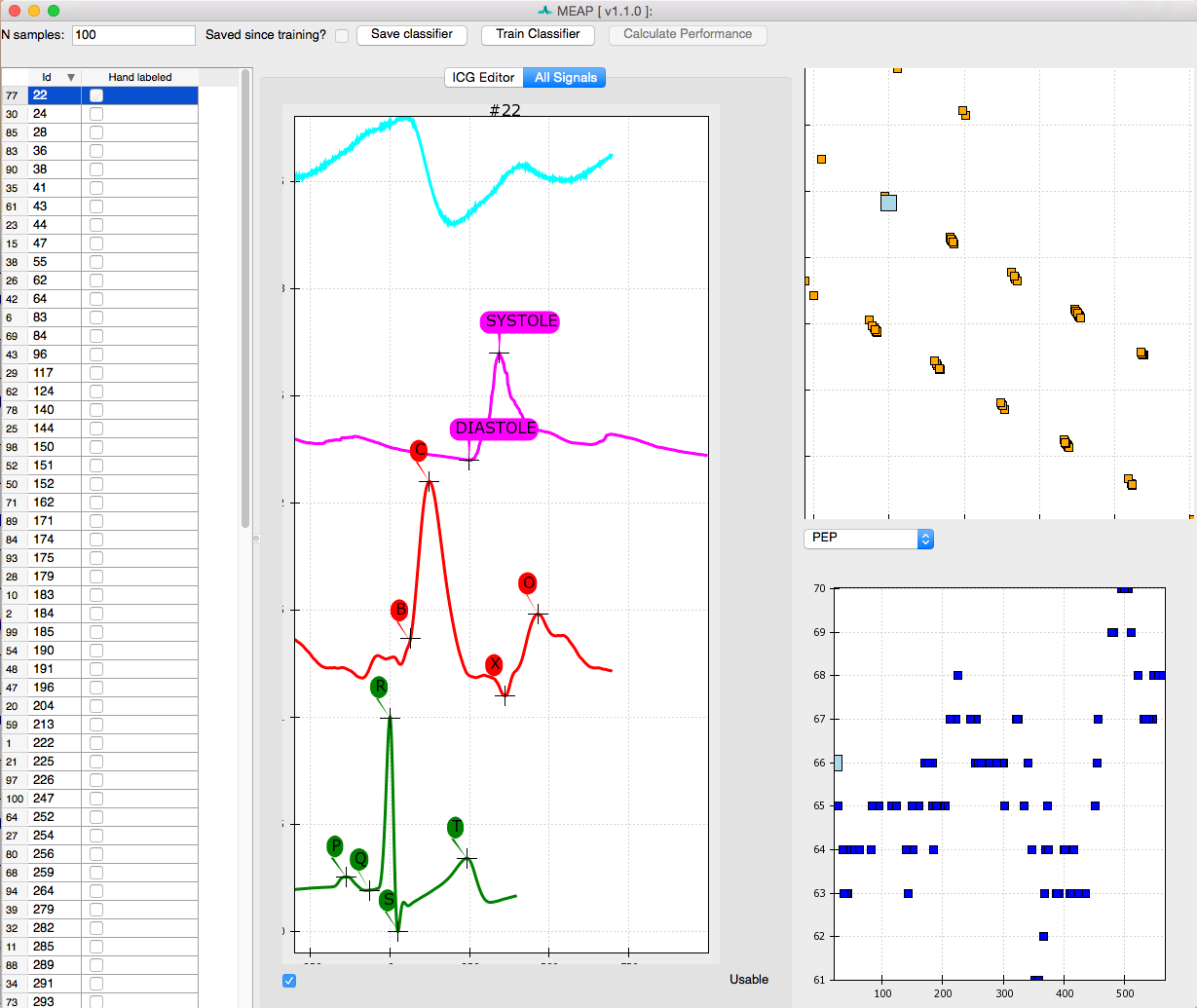
This window looks almost exactly like the one we used to mark the ensembled average points except that this time a series of randomly selected moving ensembled heart beats is listed in the left most panel. Clicking on each brings up that heart beat. Once you’ve hand labeled it, the box in that column will be checked. The top image in the top right panel displays the results of a principle components analysis of all marked inflection points. This plot allows the user to easily visualize the spread of the data and identify potential outliers. The bottom right panel plots the values for LVET, PEP, or SV, depending on which the user selects. The N samples field in the top left corner of the window allows the user to specify the number of randomly selected beats to be hand marked and employed by the classifier. If there are any beats that you wish not to include in analyses, due to noise or whatever reason, unselect the Usable box at the bottom of the window. This will remove data from this beat from all further analyses.

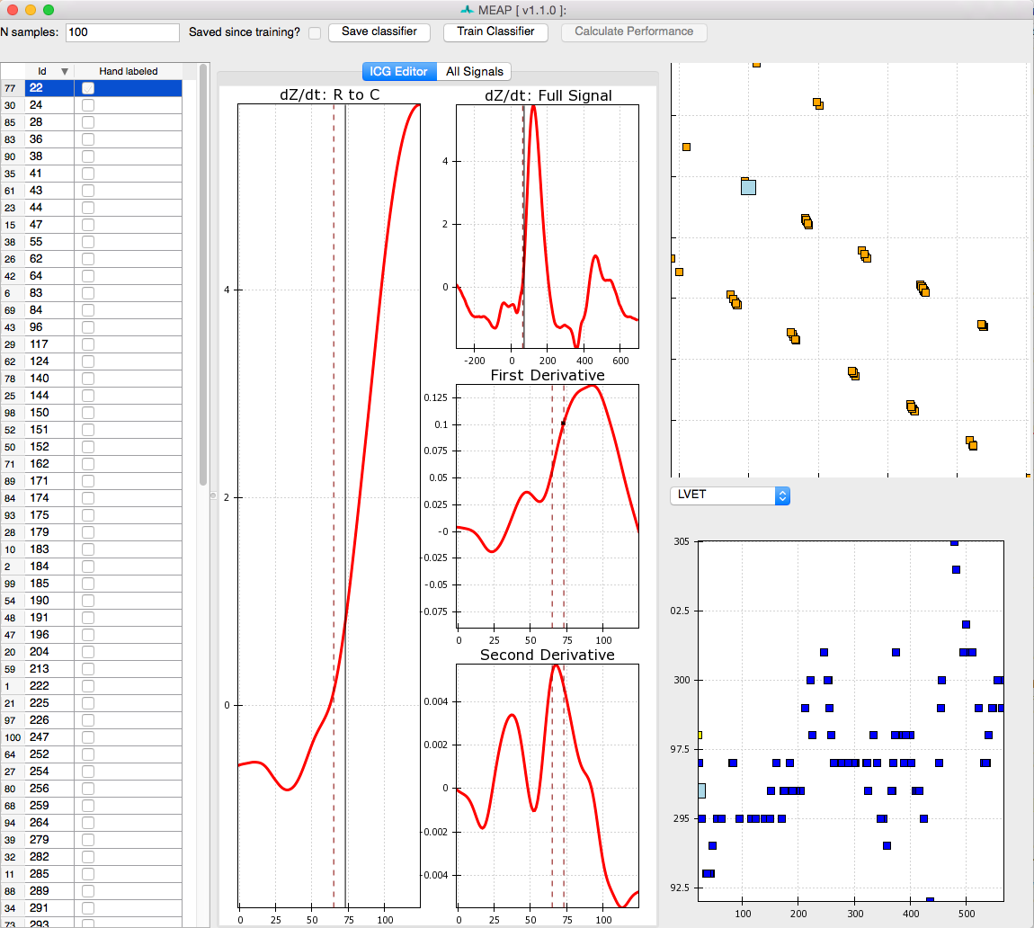
As in the Marking Custom Points stage, the user can toggle between the ICG Editor and All Signals tabs to view just the ICG signal, or all data streams together. The other aspects of this window remain the same.

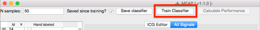
Once you are satisfied with all marked points, select Train Classifier. This may take a moment or two to process. Once complete, select Save Classifier. You can then close out of this window.

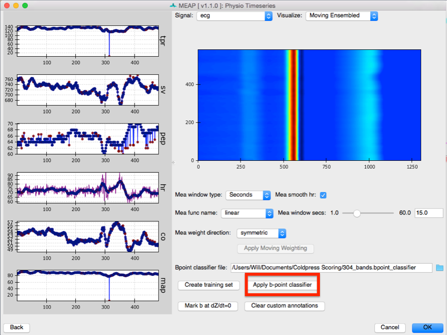
Then return to the Physio Timeseries Window. Note that the points that we hand-marked now appear in purple. The reason for MAP and TPR values dropping to zero is that blood pressure data was censored at that point. Select Apply b-point classifier.

Using SRVF-based dZ/dt registration

Starting at MEAP version 1.5 you can use SRVF-based timeseries registration. You can think of this method as similar to diffeomorphic spatial normalization used in neuroimaging group studies. Instead of manually identifying a specific region in each brain, you can warp all the brains to a template, draw the region on the template, then inverse warp the region into each individual brain. Here we’re doing the same thing with dZ/dt waveforms.

You can access this tool by clicking Register dZ/dt from the pipeline window. This process involves 4 steps. First, a single template is created from a randomly-selected subset of all heartbeats. Next, all heartbeats are registered to this initial template. Third, the warps to the initial template are used to cluster individual heartbeats into similarly-shaped subsets. A template for each of these shape “modes” is created. Finally, the user hand-marks B-Points on each mode template and these are inverse-warped to each heartbeat.

To create an initial shape template, or Karcher Mean, of your dZ/dt signals you will use the widgets in the left half of this screen:

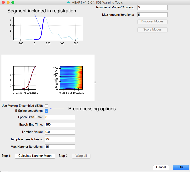
It is important to decide whether you want to use moving ensembled dZ/dt signals or the original raw signals. Original signals will vary in shape depending on the part of the respiratory cycle in which they occurred and will also have pronounced pre-load and after-load effects on the locations of the B-Points. Also, data with abrupt spikes can fail to produce a meaningful Karcher Mean. If your data has spikes, we recommend filtering it in AcqKnowledge and/or using the B-Spline smoothing option here.

Only a portion of the dZ/dt waveform is used for this procedure. Using the entire waveform causes the template-building process to be incredibly time-consuming and also produces poor results during clustering. You select the portion of the dZ/dt signal that will be included in this analysis in the Epoch Start Time and Epoch End Time fields. Lambda controls how much the time series are allowed to deform. The number of beats used and the maximum number of template-building iterations can be specified here. Once you are satisfied, click “Calculate Karcher Mean”.

After a few minutes the plots will update and the “Warp All” button will be enabled.

The updated plots will look something like the above. You will notice that the Karcher Mean (dark blue line) has higher amplitude than the global ensemble average (light blue line) and contains sharper features. These are all benefits of using an elastic time series approach. Click “Warp All” and all of your heartbeats will be registered to this initial Karcher Mean. The bottom two plots will show the individual dZ/dt signal in red after it is aligned to the Karcher Mean in blue. The image plot on the right is a heat map of the aligned dZ/dt signals.

Once all beats have been aligned to the initial Karcher Mean, you can cluster heart beats based on the similarity of their warps using the widgets in the right panel. We use the distance metrics and general procedure described in Kurtek 2017 to cluster heart beats. Choose the number of clusters and the maximum number of K-means iterations. Once satisfied with your choices, click “Detect Modes”. This will take a long time to run. If you are using MacOS, it will take much longer than any other operating system. Once completed, the “Score Modes” button will be enabled.

Clicking the “Score Modes” button will open an editor like the one below:

There will be one beat listed in the left panel for each mode you requested. Clicking on that beat will show what that cluster’s template dZ/dt looks like. The B-Point times are plotted in the upper-right panel. By editing the B-Points, the corresponding time in each original beat will be updated. Manually identify te B-Point on each Mode and the inverse warp to the original beats will be used to identify the corresponding point on the original waveform.

Once you’re satisfied, you can visit the “Compute Moving Ensembles” window again to edit individual B-Point placements.

Step 8: Process fMRI

This feature not yet functional, but coming soon.

Step 9: Save Your Preprocessed File (Again!)

Save your Work! If you have not done so already, copy the File path and paste it into the Outfile field and change the file type from .acq to .mea.mat, then click Save .meap file.

The file you just preprocessed should now be highlighted in blue. Proceed to the next file and repeat these steps until you have scored the data for all of your subjects.

To improve processing speed click the Clear Memory button to clear the memory cache before proceeding to the next file.

PART II: Calculating Ensemble and Moving Ensemble Averages

Step 1: Create a Design Spread Sheet

This should specify your subjects, your experimental design, and the path to the mea.mat files that you preprocessed:

Exactly how this file should be set up will depend on the length of the ensemble average window you are using and on other specifics of your study design.

This same file is also where your data will ultimately be printed. Thus it serves as both the input and output file for this stage of the scoring process.

Step 2: Analysis

For step 2, select Analyze on the MEAP launch window.

Ensemble Averaging

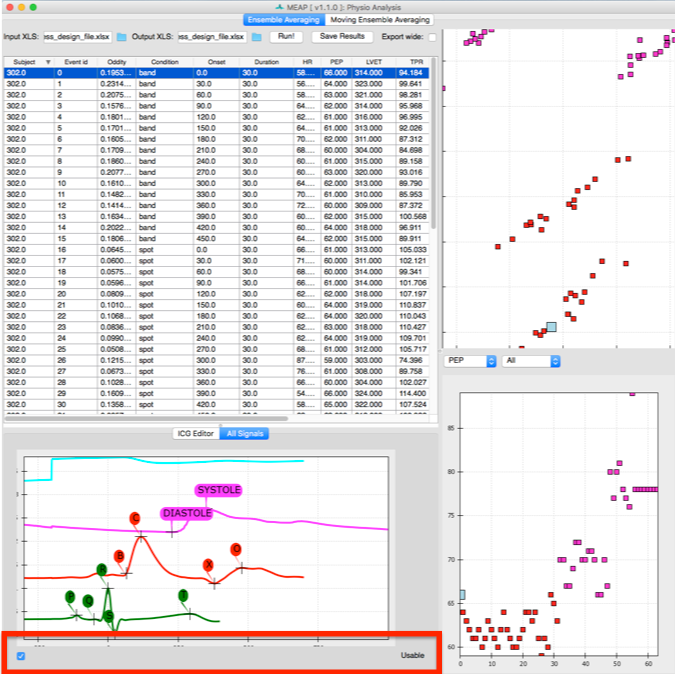
The first step is to load your prepared design file. The analyze interface will then look like this:

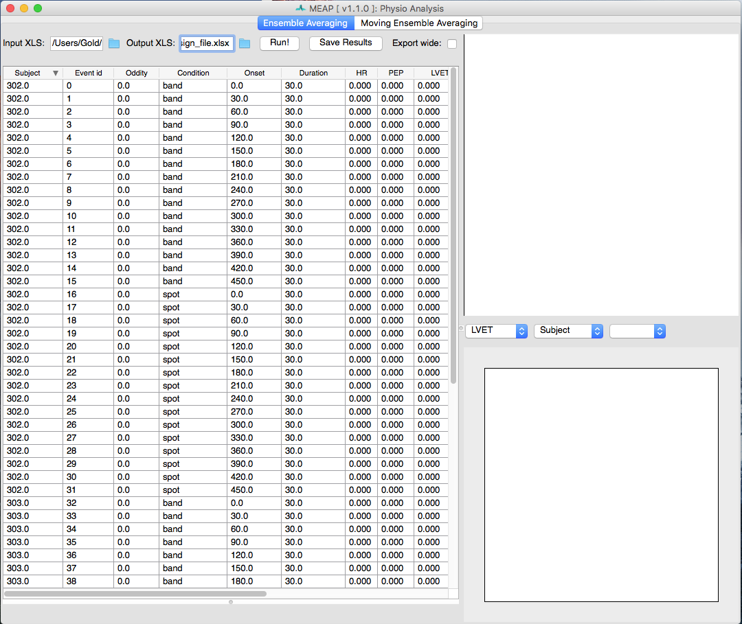
Until you click Run all values for indices will be zero and nothing will be plotted in the windows on the right. After selecting run, the interface will look something like this:

The Ensemble Average window allows the user to visualize each ensemble average (duration specified in your excel file) as well as the values for key indices (B-point, PEP, LVET) for all subjects, for a specific subject only, or for a specific data file only. In the top right corner is an ICA plot which takes all of the features of the ensemble averages into account and then plots them in two dimensions based on their covariance.

Using the column headers you can sort by subject, event, or by “oddity index” which reflects that EAs distance from the center of the ICA plot. This allows you to quickly identify problematic EAs and adjust point markings as necessary.

To view all point markings (not just the B-points) toggle the bottom window to All Signals. There you can adjust the placement of any of the inflection points. If the data for a specific EA is too noisy or you decide you don’t want to include it in analyses for whatever reason simply uncheck the Usable button at the bottom of this window and that EA will be removed from the dataset.

Using these point markings MEAP calculates the following cardiovascular indices:

1. Total Peripheral Resistance (TPR)
2. Cardiac Output (CO)
3. Stroke Volume (SV)
4. Pre-Ejection Period (PEP)
5. Mean Arterial Pressure (MAP)
6. Heart Rate (HR)
7. Heart Rate Variability (HRV)

All of these values for each EA will be exported to your excel output file:

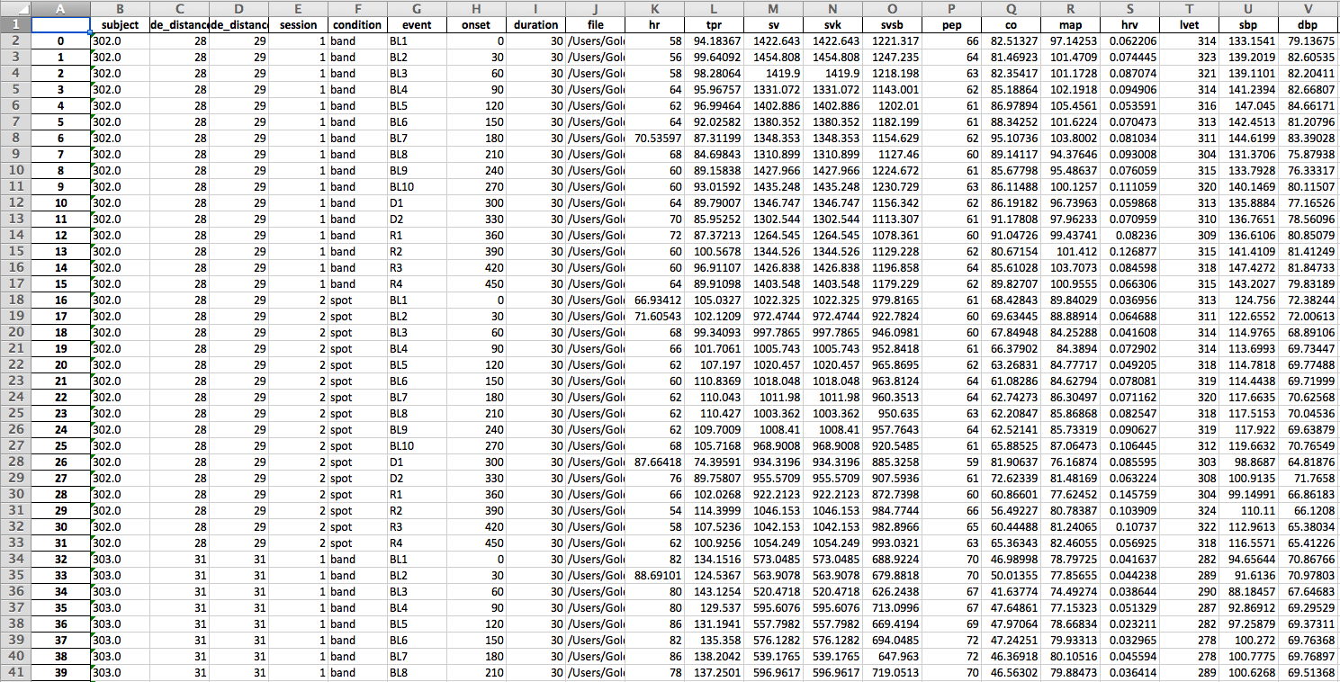
Step 3: Save Your Work!!

Click the “Save Results” button at the top of the GUI to save your work. Do this frequently as you are working. All of your custom point markings will be saved and you can reload and return to them by using the newly created output spreadsheet as input.

PART III: Analyzing your Scored Data

At this point you have completed the data scoring process. You now have a .csv file with values for each cardiovascular index for each ensemble average. MEAP calculates a slope and an intercept for each EA.

If you want to use the time series data from the moving ensemble averages computed during preprocessing, those can be pulled from the .mea.mat file using R or another statistical package of your choice.

You are now ready to move this data into whatever statistical software you prefer for analyses. Depending on what type of analyses you wish to conduct you may need to reformat the data. As it is, the data appears in long format with multiple rows of data for each subject. Some analyses require wide format where each subject has only one row of data but multiple variables for each cardiovascular index reflecting the values for each ensemble average.

Again, depending on your study design and the analyses you wish to conduct you may want to create reactivity values that reflect values for each index minus baseline values (E.g. CO_min1 - CO_BL). All analyses and data transformations are done outside of MEAP in your statistical software of choice. You should also use this software to check for outliers or any other issues with your data.